Timepicker

Following example showcases the results of different timepicking methods. For more informations, please refer to the functions documentation (vallenae.timepicker).

import time
from pathlib import Path

import matplotlib.pyplot as plt

import vallenae as vae

HERE = Path(__file__).parent if "__file__" in locals() else Path.cwd()
TRADB = HERE / "steel_plate" / "sample_plain.tradb"
TRAI = 4
SAMPLES = 2000

Read waveform from tradb

tradb = vae.io.TraDatabase(TRADB)

y, t = tradb.read_wave(TRAI)
# crop first samples
t = t[:SAMPLES]
y = y[:SAMPLES]
# unit conversion
t *= 1e6  # convert to µs
y *= 1e3  # convert to mV

Prepare plotting with time-picker results

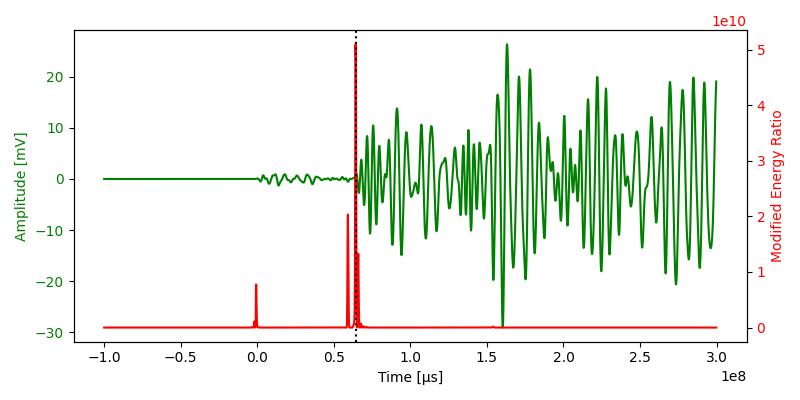
def plot(t_wave, y_wave, y_picker, index_picker, name_picker):
    _, ax1 = plt.subplots(figsize=(8, 4), tight_layout=True)
    ax1.set_xlabel("Time [µs]")
    ax1.set_ylabel("Amplitude [mV]", color="g")
    ax1.plot(t_wave, y_wave, color="g")
    ax1.tick_params(axis="y", labelcolor="g")

    ax2 = ax1.twinx()
    ax2.set_ylabel(f"{name_picker}", color="r")
    ax2.plot(t_wave, y_picker, color="r")
    ax2.tick_params(axis="y", labelcolor="r")

    plt.axvline(t_wave[index_picker], color="k", linestyle=":")
    plt.show()

Hinkley Criterion

hc_arr, hc_index = vae.timepicker.hinkley(y, alpha=5)
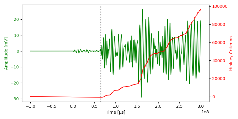
plot(t, y, hc_arr, hc_index, "Hinkley Criterion")

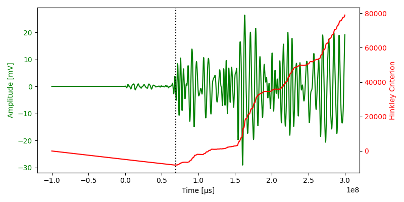
The negative trend correlates to the chosen alpha value and can influence the results strongly. Results with alpha = 50 (less negative trend):

hc_arr, hc_index = vae.timepicker.hinkley(y, alpha=50)
plot(t, y, hc_arr, hc_index, "Hinkley Criterion")

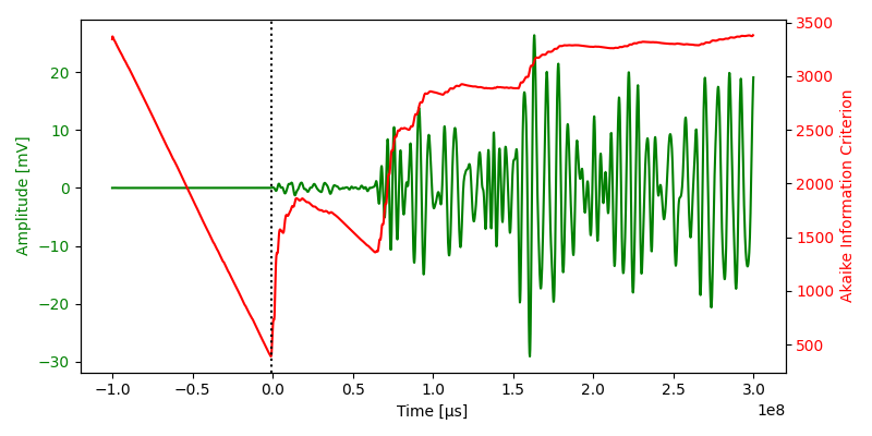
Akaike Information Criterion (AIC)

aic_arr, aic_index = vae.timepicker.aic(y)
plot(t, y, aic_arr, aic_index, "Akaike Information Criterion")

Energy Ratio

er_arr, er_index = vae.timepicker.energy_ratio(y)
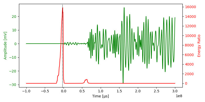
plot(t, y, er_arr, er_index, "Energy Ratio")

Modified Energy Ratio

mer_arr, mer_index = vae.timepicker.modified_energy_ratio(y)
plot(t, y, mer_arr, mer_index, "Modified Energy Ratio")

Performance comparison

All timepicker implementations are vectorized with NumPy. The average of multiple executions is reported below.

def timeit(func, loops=100):
    time_start = time.perf_counter()
    for _ in range(loops):
        func()
    return 1e6 * (time.perf_counter() - time_start) / loops  # elapsed time in µs


timer_results = {
    "Hinkley": timeit(lambda: vae.timepicker.hinkley(y, 5)),
    "AIC": timeit(lambda: vae.timepicker.aic(y)),
    "Energy Ratio": timeit(lambda: vae.timepicker.energy_ratio(y)),
    "Modified Energy Ratio": timeit(lambda: vae.timepicker.modified_energy_ratio(y)),
}

for name, execution_time in timer_results.items():
    print(f"{name}: {execution_time:0.3f} µs")

plt.figure(figsize=(8, 3), tight_layout=True)
plt.bar(timer_results.keys(), timer_results.values())
plt.ylabel("Time [µs]")
plt.show()

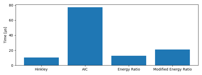
Hinkley: 17.077 µs
AIC: 74.655 µs
Energy Ratio: 17.744 µs
Modified Energy Ratio: 21.102 µs