Timepicker batch processing

Following examples shows how to stream transient data row by row, compute timepicker results and save the results to a feature database (trfdb).

from pathlib import Path
from shutil import copyfile
from tempfile import gettempdir

import matplotlib.pyplot as plt
import pandas as pd
import vallenae as vae

HERE = Path(__file__).parent if "__file__" in locals() else Path.cwd()
TRADB = HERE / "steel_plate" / "sample_plain.tradb"
TRFDB = HERE / "steel_plate" / "sample.trfdb"
TRFDB_TMP = Path(gettempdir()) / "sample.trfdb"

Open tradb (readonly) and trfdb (readwrite)

copyfile(TRFDB, TRFDB_TMP)  # copy trfdb, so we don't overwrite it

tradb = vae.io.TraDatabase(TRADB)
trfdb = vae.io.TrfDatabase(TRFDB_TMP, mode="rw")  # allow writing

Read current trfdb

print(trfdb.read())

Trf:   0%|          | 0/4 [00:00<?, ?it/s]
Trf: 100%|██████████| 4/4 [00:00<00:00, 27369.03it/s]
         FFT_CoG     FFT_FoM         PA  ...  CTP          FI          FR
trai                                     ...
1     147.705078  134.277344  46.483864  ...   11  222.672058  110.182449
2     144.042969  139.160156  59.450512  ...   35  182.291672   98.019981
3     155.029297  164.794922  33.995209  ...   55  155.191879   95.493233
4     159.912109  139.160156  29.114828  ...   29  181.023727  101.906227

[4 rows x 8 columns]

Compute arrival time offsets with different timepickers

To improve localisation, time of arrival estimates using the first threshold crossing can be refined with timepickers. Therefore, arrival time offsets between the first threshold crossings and the timepicker results are computed.

def dt_from_timepicker(timepicker_func, tra: vae.io.TraRecord):
    # Index of the first threshold crossing is equal to the pretrigger samples
    index_ref = tra.pretrigger
    # Only analyse signal until peak amplitude
    index_peak = vae.features.peak_amplitude_index(tra.data)
    data = tra.data[:index_peak]
    # Get timepicker result
    _, index_timepicker = timepicker_func(data)
    # Compute offset in µs
    return (index_timepicker - index_ref) * 1e6 / tra.samplerate

Transient data is streamed from the database row by row using vallenae.io.TraDatabase.iread. Only one transient data set is loaded into memory at a time. That makes the streaming interface ideal for batch processing. The timepicker results are saved to the trfdb using vallenae.io.TrfDatabase.write.

for tra in tradb.iread():
    # Calculate arrival time offsets with different timepickers
    feature_set = vae.io.FeatureRecord(
        trai=tra.trai,
        features={
            "ATO_Hinkley": dt_from_timepicker(vae.timepicker.hinkley, tra),
            "ATO_AIC": dt_from_timepicker(vae.timepicker.aic, tra),
            "ATO_ER": dt_from_timepicker(vae.timepicker.energy_ratio, tra),
            "ATO_MER": dt_from_timepicker(vae.timepicker.modified_energy_ratio, tra),
        }
    )
    # Save results to trfdb
    trfdb.write(feature_set)

Read results from trfdb

print(trfdb.read().filter(regex="ATO"))

Trf:   0%|          | 0/4 [00:00<?, ?it/s]
Trf: 100%|██████████| 4/4 [00:00<00:00, 80273.76it/s]
      ATO_Hinkley  ATO_AIC  ATO_ER  ATO_MER
trai
1            30.4     -1.8    -4.0     29.2
2            36.4     -0.8    -1.0     -0.4
3            67.0     -1.8    -3.2     60.4
4            65.8     -1.0    -2.2     64.2

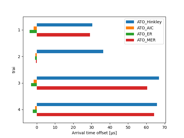
Plot results

ax = trfdb.read()[["ATO_Hinkley", "ATO_AIC", "ATO_ER", "ATO_MER"]].plot.barh()
ax.invert_yaxis()
ax.set_xlabel("Arrival time offset [µs]")
plt.show()

Trf:   0%|          | 0/4 [00:00<?, ?it/s]
Trf: 100%|██████████| 4/4 [00:00<00:00, 87838.83it/s]

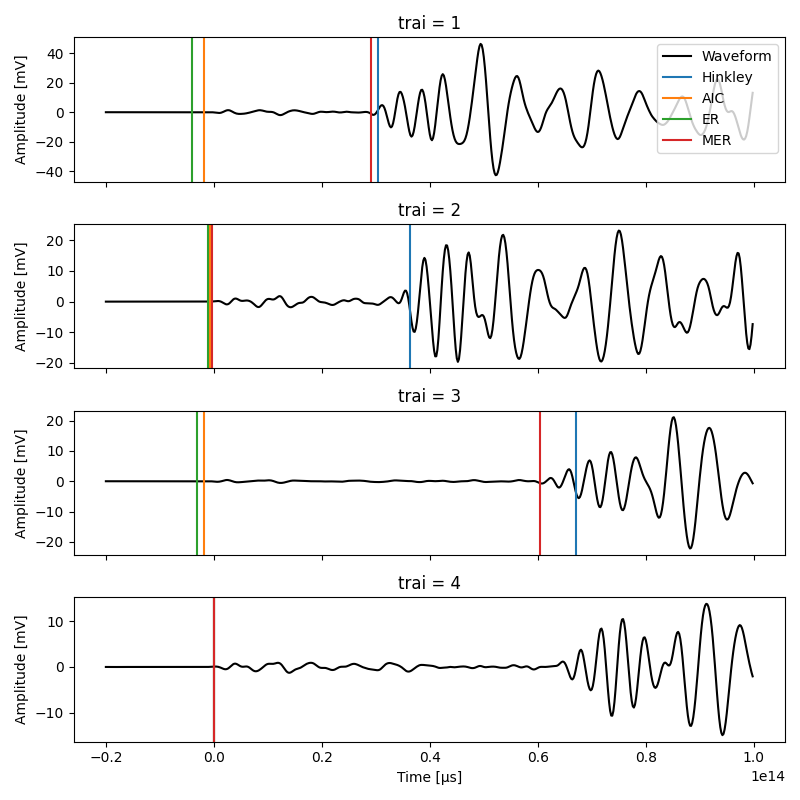
Plot waveforms and arrival times

_, axes = plt.subplots(4, 1, tight_layout=True, figsize=(8, 8))
for row, ax in zip(trfdb.read().itertuples(), axes):
    trai = row.Index

    # read waveform from tradb
    y, t = tradb.read_wave(trai)

    # plot waveform
    ax.plot(t[400:1000] * 1e6, y[400:1000] * 1e3, "k")  # crop and convert to µs/mV
    ax.set_title(f"trai = {trai}")
    ax.set_xlabel("Time [µs]")
    ax.set_ylabel("Amplitude [mV]")
    ax.label_outer()
    # plot arrival time offsets
    ax.axvline(row.ATO_Hinkley, color="C0")
    ax.axvline(row.ATO_AIC, color="C1")
    ax.axvline(row.ATO_ER, color="C2")
    ax.axvline(row.ATO_MER, color="C3")

axes[0].legend(["Waveform", "Hinkley", "AIC", "ER", "MER"])
plt.show()

Trf:   0%|          | 0/4 [00:00<?, ?it/s]
Trf: 100%|██████████| 4/4 [00:00<00:00, 68200.07it/s]

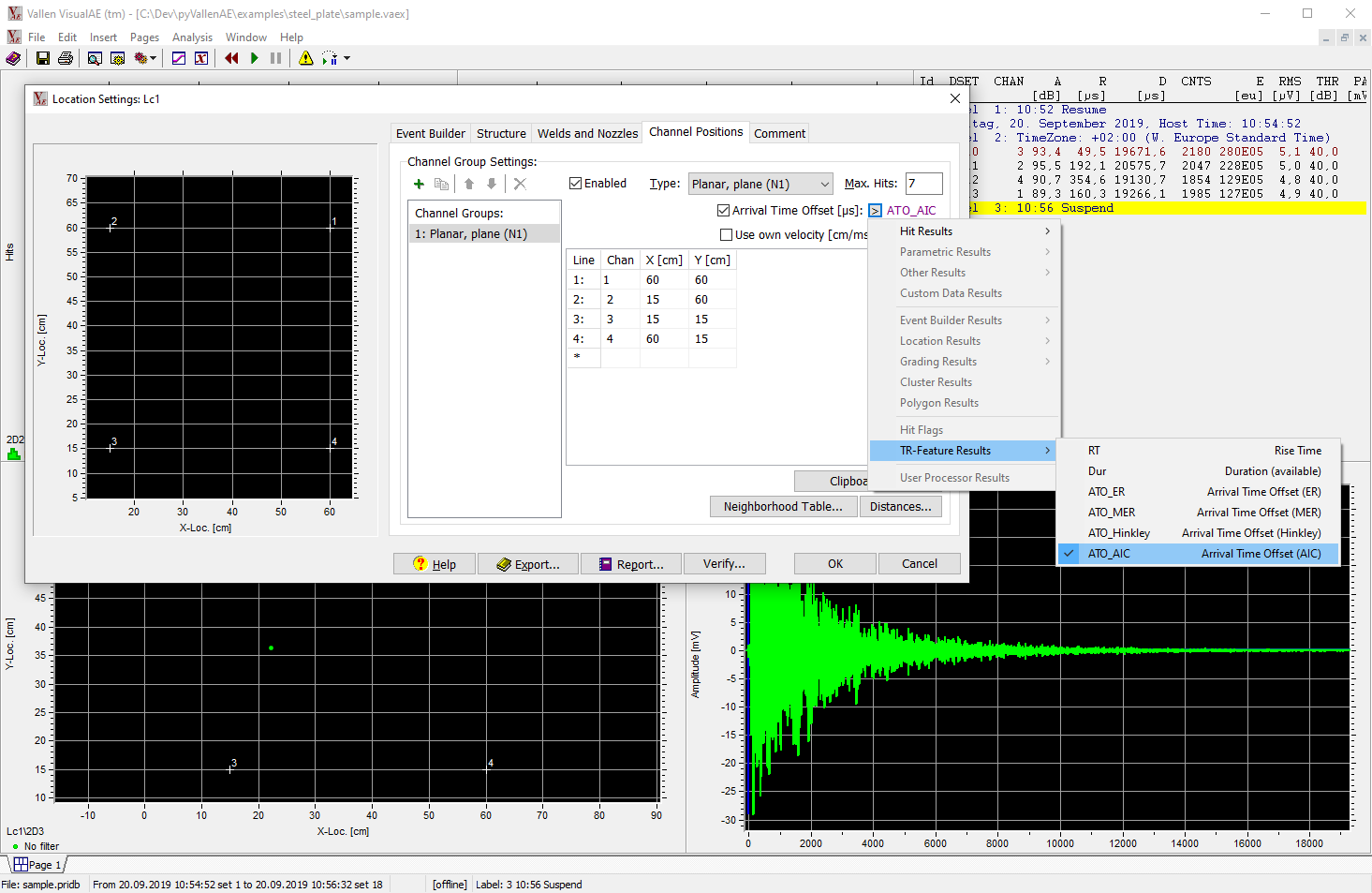
Use results in VisualAE

The computed arrival time offsets can be directly used in VisualAE. We only need to specify the unit. VisualAE requires them to be in µs. Units and other column-related meta data is saved in the trf_fieldinfo table. Field infos can be retrieved with vallenae.io.TrfDatabase.fieldinfo:

print(trfdb.fieldinfo())

{'FFT_CoG': {'SetTypes': 2, 'Unit': '[kHz]', 'LongName': 'F(C.o.Gravity)', 'Description': 'Center of gravity of spectrum', 'ShortName': None, 'FormatStr': None}, 'FFT_FoM': {'SetTypes': 2, 'Unit': '[kHz]', 'LongName': 'F(max. Amp.)', 'Description': 'Frequency of maximum of spectrum', 'ShortName': None, 'FormatStr': None}, 'PA': {'SetTypes': 8, 'Unit': '[mV]', 'LongName': 'Peak Amplitude', 'Description': None, 'ShortName': None, 'FormatStr': None}, 'RT': {'SetTypes': 8, 'Unit': '[µs]', 'LongName': 'Rise Time', 'Description': None, 'ShortName': None, 'FormatStr': None}, 'Dur': {'SetTypes': 8, 'Unit': '[µs]', 'LongName': 'Duration (available)', 'Description': None, 'ShortName': None, 'FormatStr': None}, 'CTP': {'SetTypes': 8, 'Unit': None, 'LongName': 'Cnts to peak', 'Description': None, 'ShortName': None, 'FormatStr': '#'}, 'FI': {'SetTypes': 8, 'Unit': '[kHz]', 'LongName': 'Initiation Freq.', 'Description': None, 'ShortName': None, 'FormatStr': None}, 'FR': {'SetTypes': 8, 'Unit': '[kHz]', 'LongName': 'Reverberation Freq.', 'Description': None, 'ShortName': None, 'FormatStr': None}}

Show results as table:

print(pd.DataFrame(trfdb.fieldinfo()))

                                   FFT_CoG  ...                   FR
SetTypes                                 2  ...                    8
Unit                                 [kHz]  ...                [kHz]
LongName                    F(C.o.Gravity)  ...  Reverberation Freq.
Description  Center of gravity of spectrum  ...                 None
ShortName                             None  ...                 None
FormatStr                             None  ...                 None

[6 rows x 8 columns]

Write units to trfdb

Field infos can be written with vallenae.io.TrfDatabase.write_fieldinfo:

trfdb.write_fieldinfo("ATO_Hinkley", {"Unit": "[µs]", "LongName": "Arrival Time Offset (Hinkley)"})
trfdb.write_fieldinfo("ATO_AIC", {"Unit": "[µs]", "LongName": "Arrival Time Offset (AIC)"})
trfdb.write_fieldinfo("ATO_ER", {"Unit": "[µs]", "LongName": "Arrival Time Offset (ER)"})
trfdb.write_fieldinfo("ATO_MER", {"Unit": "[µs]", "LongName": "Arrival Time Offset (MER)"})

print(pd.DataFrame(trfdb.fieldinfo()).filter(regex="ATO"))

                               ATO_Hinkley  ...                    ATO_MER
SetTypes                              None  ...                       None
Unit                                  [µs]  ...                       [µs]
LongName     Arrival Time Offset (Hinkley)  ...  Arrival Time Offset (MER)
Description                           None  ...                       None
ShortName                             None  ...                       None
FormatStr                             None  ...                       None

[6 rows x 4 columns]

Load results in VisualAE

Time arrival offsets can be specified in the settings of Location Processors - Channel Positions - Arrival Time Offset. (Make sure to rename the generated trfdb to match the filename of the pridb.)